GLMMs with Cersei Lannister
2016-09-15
I wrote this a long time ago while preparing for job interviews. Though I’ve made some stylistic changes, the analysis is as it was when I first published it on a previous blog. In other words, nothing in this post relates to my current projects at Google, nor were any Google data used or consulted: it was written over a year before my start date. All methods and applications covered are commonplace, and are discussed widely and publicly.
This post does the following:
- Gives accessible examples of fitting mixed-effects models in R
- Discusses the interpretation of and motivation for mixed effects regression models
- Provides short, educational GOT fan-fic, with pictures
Some of this is in response to a great article from folks at Google. They show a cool result about the predictive efficacy of a mixed-effects model, so I decided to try a related experiment. I found their interpretation of the model somewhat off, particularly in distinguishing it from a Bayesian approach. So I’ll be expanding on that as well.
Some code is in-line, but not all of it. The code provided is associated with the R library chosen to fit the mixed models, called lme4, and is meant to display its basic functionality. The rest of the code is available upon request.
Hat tip to this neat tool providing endless Westeros-style names to use for the first story. That story covers what it means to have different experimental units in a regression model. This is an important concept for understanding why we might want to use a mixed-model in the first place. Enter the Lannister family:
Jaime’s archers
Jaime was preparing for a long journey, on official Lannister business. Knowing that things would likely come to swords, he assembled a small force to accompany him. He had some time to take special care outfitting his troops, so he decided to run an experiment with two different kinds of bows.
Normally, Lannister forces used bows made from Northwood, as common knowledge said they are stronger than Southwood bows. However, since Jaime is a Southerner, he preferred Southwood bows out of pride and convenience. He wanted to see if use of Southwood bows cause a statistically significant difference in archer range.
So, he chose three archers randomly from the kingdom’s forces, who each would shoot a Northwood bow and a Southwood bow 10 times. He bullied some local city-folk into measuring and recording the distance of the shots, in meters. Some of the resulting data is shown below:
##   Distance_      Bow_          Name_
## 1       163 Northwood Deonte Skinner
## 2       163 Northwood Deonte Skinner
## 3       159 Northwood Deonte Skinner
## 4       149 Northwood Deonte Skinner
## 5       152 Northwood Deonte Skinner
## 6       155 Northwood Deonte Skinner
The other two archers were named Fabiar Darklyn and Margan Drumm. Jaime fit the following linear regression model to his experiment’s data: \[ Y_{ik} = \mu + \tau\mathbb{1}(i = 2) + \epsilon_{ik} \] In that equation, \(Y_{ik}\) is the \(k\)-th shot from bow \(i = 1,2\), and the Southwood bow is considered to be the second bow. The variables \(\mu\) and \(\tau\) represent the mean shot distance and mean effect of the Southwood bow. The final term \(\epsilon_{ik}\) is the random error (the Winds of Westeros, perhaps) contributing to the \(k\)-th shot from the \(i\)-th bow. There are \(3\times 10 = 30\) shots per bow, since each marksman shoots each bow 10 times. The errors are independent shot-to-shot and Normally distributed with constant variance \(\sigma^2_e\). Here’s the summary of Jaime’s analysis:
lm0 <- lm(Distance_ ~ Bow_, data = JaimeExp1$Data)
summary(lm0)
##
## Call:
## lm(formula = Distance_ ~ Bow_, data = JaimeExp1$Data)
##
## Residuals:
## Min 1Q Median 3Q Max
## -25.84 -15.59 -10.21 23.75 34.70
##
## Coefficients:
## Estimate Std. Error t value Pr(>|t|)
## (Intercept) 167.885 3.678 45.643 <2e-16 ***
## Bow_Southwood -9.767 5.202 -1.878 0.0655 .
## ---
## Signif. codes: 0 '***' 0.001 '**' 0.01 '*' 0.05 '.' 0.1 ' ' 1
##
## Residual standard error: 20.15 on 58 degrees of freedom
## Multiple R-squared: 0.0573, Adjusted R-squared: 0.04105
## F-statistic: 3.526 on 1 and 58 DF, p-value: 0.06546When the archers switched to a Southwood bow, their shot distances decreased by about 10 meters, on average. However, Jaime realized his p-value was not below that magical 0.05 threshold! He strutted merrily out of the experiment grounds, confident that his results must be due to unfair winds. (Clearly, Jaime missed some important Statistical Lectures of the Crown.)

“A Lannister always pays attention to statistical differences in bow types”
Adding archer terms
He was, of course, stopped by his brother Tyrion, who said “now Jaime, can’t you see that you chose archers of wildly different statures? Only a fool would not account for this in his analysis.” Grumpily, Jaime re-fit his model with additional terms for the archers:
\[ Y_{ijk} = \mu + \tau\mathbb{1}(i = 2) + \alpha_j + \epsilon_{ik} \]
Here, \(Y_{ijk}\) is the \(k\)-th shot (now \(k\) goes from 1 to 10) from the \(j\)-th archer using the \(i\)-th bow. The \(\alpha_j\) parameters represent archer \(j\)’s baseline skill. Here were Jaime’s results with the new model:
lm1 <- lm(Distance_ ~ Bow_ + Name_, data = JaimeExp1$Data)
summary(lm1)
##
## Call:
## lm(formula = Distance_ ~ Bow_ + Name_, data = JaimeExp1$Data)
##
## Residuals:
## Min 1Q Median 3Q Max
## -10.1652 -3.4554 -0.5064 2.5754 13.1611
##
## Coefficients:
## Estimate Std. Error t value Pr(>|t|)
## (Intercept) 156.427 1.238 126.386 < 2e-16 ***
## Bow_Southwood -9.767 1.238 -7.891 1.17e-10 ***
## Name_Fabiar Darklyn 38.585 1.516 25.454 < 2e-16 ***
## Name_Margan Drumm -4.212 1.516 -2.779 0.00741 **
## ---
## Signif. codes: 0 '***' 0.001 '**' 0.01 '*' 0.05 '.' 0.1 ' ' 1
##
## Residual standard error: 4.794 on 56 degrees of freedom
## Multiple R-squared: 0.9485, Adjusted R-squared: 0.9457
## F-statistic: 343.6 on 3 and 56 DF, p-value: < 2.2e-16After accounting for the different archer, the estimated effect of the Southwood bow became quite statistically significant. These results weren’t as pleasing to Jaime, who stormed past a smirking Tyrion. “Well? What read your results?” he heard as he slammed the training field gate behind him.
So what happened? There were two separable sources of error around the bow effect: per-shot random error, and variance among archer shooting strengths. At Tyrion’s suggestion, Jaime controlled for this in the second model by including archer effects.

“I drink, and I account for variance in experimental units”
Here’s an illustration of why it’s important to include archer effects, or in general, “experimental unit” effects. Without knowledge of the particular archer, Jaime’s data look like this:
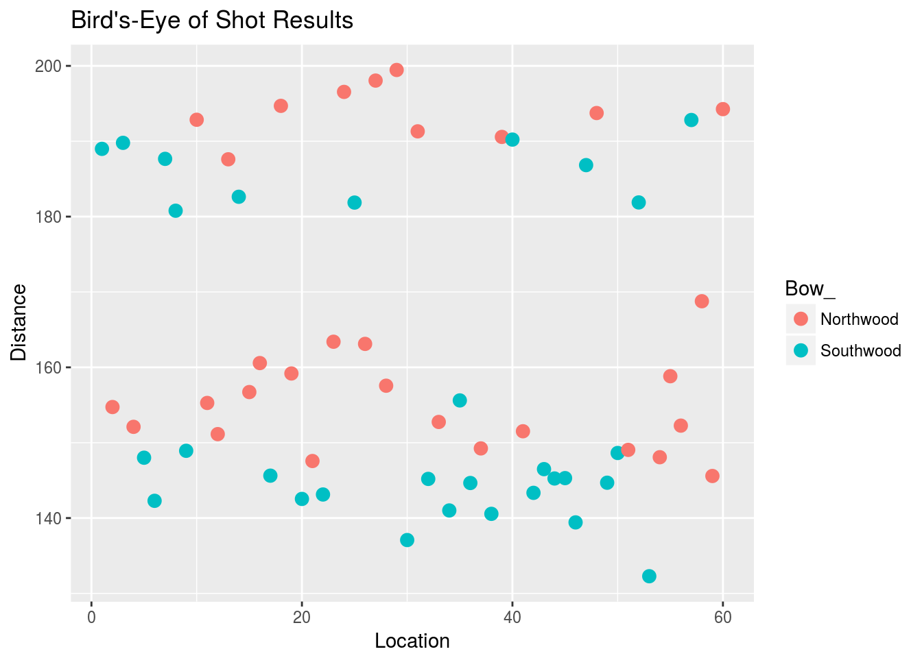
The red shots look somewhat above the blue shots, but the shot points seem to be layered. Here’s the plot with points shaped differently for different archers:
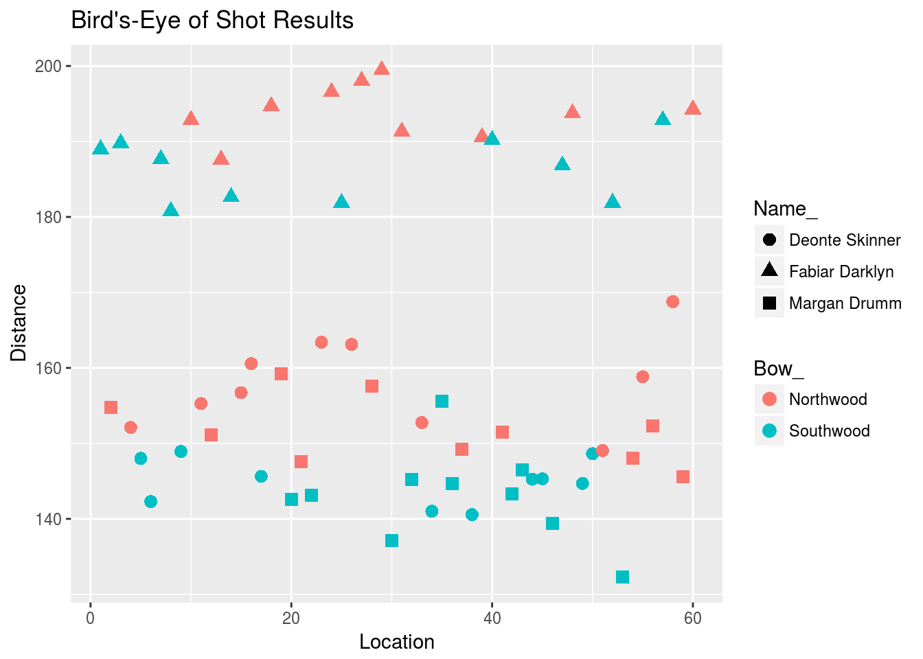
It’s now apparent that the red shots are usually higher than the green shots, and the shots cluster around distinct locations that depend on the marksman. Including marksman terms in the model allows for estimation of the noise variance around the marksman centers, rather than the overall center. This is beneficial from (at least) two standpoints:
- Interpretation: the variance due to archer skill is clearly not random error, so a model that does not account for the marksman will give an inaccurate estimate of the true per-shot variance.
- Estimation of \(\tau\): we are better able to “see” the effect of the Southwood bow when we separate the shots by marksman.
After cooling down a little, Jaime realized that, despite not achieving the result he wanted, his findings could be useful to the Lannister army. He decided to run a larger experiment with 50 archers to solidify the results. Here was the outcome:
lm2 <- lm(Distance_ ~ Bow_ + Name_, data = JaimeExp2$Data)
summary(lm2)
##
## Call:
## lm(formula = Distance_ ~ Bow_ + Name_, data = JaimeExp2$Data)
##
## Residuals:
## Min 1Q Median 3Q Max
## -15.4424 -3.3524 -0.1689 3.2859 14.8538
##
## Coefficients:
## Estimate Std. Error t value Pr(>|t|)
## (Intercept) 168.8198 1.1263 149.883 < 2e-16 ***
## Bow_Southwood -10.4792 0.3154 -33.221 < 2e-16 ***
## Name_Aldo Apperford -12.2736 1.5772 -7.782 1.86e-14 ***
## Name_Antorn Feller 34.5155 1.5772 21.884 < 2e-16 ***
## Name_Arren Durrandon 29.3949 1.5772 18.637 < 2e-16 ***
## Name_Ashtin Orme 11.5839 1.5772 7.345 4.44e-13 ***
## Name_Barret Foral -16.6079 1.5772 -10.530 < 2e-16 ***
## Name_Barrock Ryswell 6.4531 1.5772 4.091 4.65e-05 ***
## Name_Brack Mallister -53.4039 1.5772 -33.860 < 2e-16 ***
## Name_Brandeth Erenford 6.1860 1.5772 3.922 9.41e-05 ***
## Name_Brayan Trante -35.2405 1.5772 -22.344 < 2e-16 ***
## Name_Charres Apperford 0.3317 1.5772 0.210 0.833494
## Name_Clarrik Parge 8.2105 1.5772 5.206 2.37e-07 ***
## Name_Codin Sadelyn 37.8102 1.5772 23.973 < 2e-16 ***
## Name_Culler Vyrwel 6.8461 1.5772 4.341 1.57e-05 ***
## Name_Curtass Shiphard -33.6791 1.5772 -21.354 < 2e-16 ***
## Name_Denzin Garner -21.6985 1.5772 -13.758 < 2e-16 ***
## Name_Deran Swygert 5.3668 1.5772 3.403 0.000695 ***
## Name_Donnal Brackwell -18.5525 1.5772 -11.763 < 2e-16 ***
## Name_Dontar Brask 3.0880 1.5772 1.958 0.050534 .
## Name_Dran Kenning -4.3976 1.5772 -2.788 0.005406 **
## Name_Dwan Plumm -14.3560 1.5772 -9.102 < 2e-16 ***
## Name_Eddard Meadows -24.9352 1.5772 -15.810 < 2e-16 ***
## Name_Erock Conklyn 11.5451 1.5772 7.320 5.28e-13 ***
## Name_Evin Rane -33.1439 1.5772 -21.014 < 2e-16 ***
## Name_Fabiar Darklyn -33.2426 1.5772 -21.077 < 2e-16 ***
## Name_Harden Blest -30.0566 1.5772 -19.057 < 2e-16 ***
## Name_Howar Clifton -2.6749 1.5772 -1.696 0.090221 .
## Name_Jaesse Cantell -15.7270 1.5772 -9.971 < 2e-16 ***
## Name_Jares Grell 3.6472 1.5772 2.312 0.020966 *
## Name_Jarvas Bywater 8.6005 1.5772 5.453 6.32e-08 ***
## Name_Jeffary Mudd -4.4122 1.5772 -2.797 0.005254 **
## Name_Jeran Parsin -8.9081 1.5772 -5.648 2.14e-08 ***
## Name_Kober Maeson -5.4609 1.5772 -3.462 0.000559 ***
## Name_Koryn Staunton 32.5297 1.5772 20.625 < 2e-16 ***
## Name_Marak Herston -51.0331 1.5772 -32.357 < 2e-16 ***
## Name_Mikal Netley -11.2779 1.5772 -7.151 1.72e-12 ***
## Name_Mykal Ryser -21.1308 1.5772 -13.398 < 2e-16 ***
## Name_Nelsor Baxter -19.2805 1.5772 -12.225 < 2e-16 ***
## Name_Portar Parge 36.7979 1.5772 23.331 < 2e-16 ***
## Name_Raman Brakker 36.6719 1.5772 23.251 < 2e-16 ***
## Name_Randar Condon -4.3076 1.5772 -2.731 0.006428 **
## Name_Roberd Spyre 3.6156 1.5772 2.292 0.022098 *
## Name_Rolan Morrass 25.9665 1.5772 16.464 < 2e-16 ***
## Name_Samn Whitehill -18.9911 1.5772 -12.041 < 2e-16 ***
## Name_Sarrac Ridman -9.2904 1.5772 -5.890 5.34e-09 ***
## Name_Seamas Knigh 3.9833 1.5772 2.526 0.011713 *
## Name_Seldan Harker -21.1080 1.5772 -13.383 < 2e-16 ***
## Name_Sharun Mudd -27.9034 1.5772 -17.692 < 2e-16 ***
## Name_Zandren Kneight -53.3039 1.5772 -33.797 < 2e-16 ***
## Name_Zarin Goodbrother -21.9110 1.5772 -13.892 < 2e-16 ***
## ---
## Signif. codes: 0 '***' 0.001 '**' 0.01 '*' 0.05 '.' 0.1 ' ' 1
##
## Residual standard error: 4.988 on 949 degrees of freedom
## Multiple R-squared: 0.9585, Adjusted R-squared: 0.9564
## F-statistic: 438.8 on 50 and 949 DF, p-value: < 2.2e-16Having disregarded much of his scientific education, Jaime felt quite overwhelmed with this massive list of parameter estimates. In particular, he was confused by the few archers without a statistically significant estimate. Should he re-run the experiment without them? (Note, the standard errors for the archer effect estimates are the same because they all fired the same number of shots.)
This time, Cersei was hanging around the training grounds. Overhearing Jaime, she decided to step in. “Jaime, don’t trouble yourself with those worrisome parameter estimates for the archers. I looked at your charts from the first experiment. It is certainly proper to account for archers in the model, but the only value we care about is the variance of their skills.” Later that afternoon she developed Westeros’s first Linear Mixed Effects model. In this model, archer effects are considered to be random draws from a larger population.

“With these equations I shall secure the reputation of the Lannister name in both might and maths”
The mixed-effects model and sources of randomness
Cersei’s key observation is that Jaime chose 50 archers out of the large population of archers in and around King’s Landing. Furthermore, he did so in a random fashion, distributing the bow test across a representative population of archers. This randomness can be incorporated in the model by treating archer effects as Normal random variables with a common, fixed variance: \[ Y_{ijk} = \mu + \tau\mathbb{1}(i = 2) + \alpha_j + \epsilon_{ik}\;\;\;\;\;\;\;\;\;\;\;\;\;\;\alpha_j\sim\mathcal{N}(0, \sigma^2_a) \] The \(\alpha_j\)’s are now not of interest to estimate; they exist to separate out the contribution of marksman skill to per-shot variance. This “variance component”, \(\sigma^2_a\), is now the archer parameter of interest.
Note that, though the \(\alpha_j\)’s as modeled as random variables, they do not change shot-to-shot. Mechanistically, they are still fixed features of the archer. We regard them as random only to focus on the underlying distribution of archer skill, and its effect on the predictive model.
Random-effects vs. Bayesian randomness
Wait, if the parameters are random, isn’t this a Bayesian model? A reasonable question. In my view, the parameters in a mixed model get their randomness from the unit (marksman) sampling process, so they have objective randomness, because there is a real population of parameters being sampled from. In a Bayesian model, however, parameters have subjective randomness in the sense that their prior and posterior distributions are meant to quantify our personal uncertainty about their values.
These are distinct conceptions of randomness. In fact, it is possible to model the random effects in a mixed-effects model as, additionally, subjectively random with respect to their values (called Bayesian Linear Mixed Models). So, we can fit either a fixed-effects or a mixed-effects model, each with a fully Bayesian approach, or not. The choice to employ a mixed-effects model in the first place still exists in the Bayesian framework, and depends on all the same aspects of our modeling goals.
Look back at the full fixed-effects model we considered for the bow experiments. In the most straightforward Bayesian framework, we would specify a conjugate set of of priors distributions: Normal for \(\mu\), \(\tau\), and the \(\alpha_j\)’s, and Inverse Gamma for \(\sigma^2_e\).
For the full mixed-effects model, however, it sort of looks like we already have a prior on the \(\alpha\text{'s}\). I would argue that this is an abuse of the term “prior”. The Normal distribution on the \(\alpha\text{'s}\) still represents the sampling uncertainty in the model. In our Gibbs sampler, it is used to update the \(\alpha\text{'s}\), but if we store the \(\alpha\text{'s}\) what we end up with should not be interpreted as a posterior distribution of a fixed parameter.
This is not just a semantic difference: in the Bayesian approach to our mixed-effects model, we would need a prior on \(\sigma^2_a\), since that is the archer parameter of interest. In the Bayesian fixed-effects model, we gave the \(\alpha\text{'s}\) Normal priors directly, and \(\sigma^2_a\) was a fixed hyperparameter.
But the semantic distinctions are important too. It would be inappropriate, for instance, to talk about Bayes Factors or credible intervals associated with the \(\alpha\text{'s}\), since from a modeling perspective we have decided not to treat them as values to estimate or do inference on.
When not to use a mixed-effects model
What’s special about this sampling situation? Aren’t we always picking experimental units out of a larger population? Yes, but we don’t always do so randomly. Often, we care about particular units of interest that we already know about before the experiment, so we pick them directly. There’s nothing random about this process. Also, if we have that sort of interest in the units, usually estimating their effects is an important goal of the analysis, in which case we should not model the effects as random.
Going back to the story on this, Jaime might care to also estimate the skills of a few archers he knows about. In this case, he’d probably hand-pick fewer archers, and have them take more shots.
As a more realistic example, consider a small school district doing a standardized test analysis on their three middle schools. There will be many, many observations from each middle school, and the district is not necessarily interested in considering the larger population of middle schools. Their aim is to build a predictive model for their particular district, and do inference on parameters for their schools only.
Fitting the mixed-effects model
Let’s fit the model to Jaime’s 2nd set of experimental data:
lme2 <- lmer(Distance_ ~ Bow_ + (1 | Name_), data = JaimeExp2$Data)The switch to mixed effects modeling shifts the focus from inference on the individual archer to inference on the population of archers. This focus is important in applications from many fields, like biology (where observations may come from many organisms), economics (where observations may come from many regions or agents), or clinical trials (where observations may come from many different labs). In our example, it makes sense for Cersei to want to learn about the variance in city-wide marksman skill along with the effect of Southbows. The estimate \(\hat\sigma^2_a\) gives her this:
VarCorr(lme2)## Groups Name Std.Dev.
## Name_ (Intercept) 22.9698
## Residual 4.9875confint(lme2)[1:2, ]## 2.5 % 97.5 %
## .sig01 18.907078 28.054556
## .sigma 4.768896 5.217741The output above gives the estimates for \(\sigma_a\) and \(\sigma_e\), and the assocated confidence intervals. These parameters don’t exist in a fixed-effects model.
Using the model to choose archer
“But wait,” Jaime might protest, “what if I care about the particular archer I happened to put to task? Now we know that Northwood bows are the obvious choice, how does our model help me choose which men to take on my journey? Cersei’s model isn’t specific enough. At least with the fixed effects model I had parameter estimates!”
Actually, a mixed effects model can rank the units (archers) in an analogous way. Once the model is fit, we can calculate the conditional expectation of a particular archer’s effect, given their experimental data. This can operate as a skill score for the archer: \[ \text{Score for archer }j = \mathbb{E}\left[\alpha_j | \bar y_{j\cdot}\right] \] Above, \(\bar y_{j\cdot}\) is the \(j\)-th archer’s average shot distance. Remember, in the model, each \(\alpha_j\) is random, with mean zero. So taking expectations shouldn’t seem useful, at first. However, knowledge of the experimental data biases the expectation of \(\alpha_j\), depending on where the data fall relative to the overall mean. The above quantity is often taken as a “predictor” of \(\alpha_j\), and archers with higher \(\bar y_{j\cdot}\)’s have higher predictions.
As it turns out, these predictions are exactly proportional to archer-wise parameter estimates from the fixed-effects model. So Jaime isn’t losing anything! Also, since he’s planning for a journey, the “prediction” interpretation is nice.
These characteristics of mixed-effects models are part of Bayesian approach, as well. We can compute posterior conditional means for the \(\alpha\text{'s}\), and examine the posterior distributions for \(\mu\), \(\tau\), and the variance components. The choice between mixed-effects and fixed-effects modeling has little to do with the choice between a frequentist and Bayesian approach to parameter estimation.
What about \(\tau\)?
At least for vanilla linear models, parameter and standard error estimates for fixed effects in the mixed model are the same as what they would be in the full fixed-effects model fit. However, for massive data sets with lots of parameters, it’s standard practice nowadays to use a penalized likelihood, like LASSO or RIDGE. As such, the authors of the Google blog post compared mixed-effects models and penalized linear models, and found that the mixed-effects model had slightly higher predictive power.
One explanation for this could be that shrinking experimental unit effect estimates isn’t optimal for predictive purposes. For example, though many archer parameters in Jaime’s fixed-effects model weren’t significant, it was still useful to account for their un-penalized values (see the exploratory plots with just three archers). The mixed-effect model does this by implicitly retaining the archer-wise predicted parameters, but a LASSO-penalized fixed-effect model won’t.
Let’s see how all this plays out with a much larger data set.
A larger-scale example
Suppose you work for a company that provides online services with accompanying ads. Your team is trying to decide between two versions of a general ad display module for a webpage. The metric for display effectiveness is the proportion of times a user interacts with (“clicks-through”) the ad out of the number of times they see it (“impressions”). Higher click-through rate (CTR) is good because it means companies who pay for ad placement will pay more.
An appropriate model for this situation is a logistic regression. In this model, each user \(j\) encounters the \(i\)-th version of the display \(n_{ij}\) times, and has some probability \(p_{ij}\) of clicking on some part of it each time. This \(p_{ij}\) will depend on which version of the display user \(j\) is currently in front of. The parameter \(\tau\) will represent the fixed effect of the new display version, analogous to the Southwood bow. The \(\alpha_j\)’s will be each user’s “clickiness” effect, and is analogous to archer skill.
In this example, let’s add another simulation component generating the total number of impressions \(n_{ij}\) at random from a Poisson distribution with \(\lambda = 20\). Also, we need a coin flip variable which chooses the “treatment” users. Finally, I diverted a (randomly chosen) latter portion of the treatment users’ impressions to the second display.
If we assume we already know each impression count \(n_{ij}\), the simulation model is: \[ Y_{ij}\sim\text{Binomial}(p_{ij}, n_{ij}),\;\;\;\;\;\;\log\left(\frac{p_{ij}}{1 - p_{ij}}\right) = \mu + \tau\mathbb{1}(i = 2) + \alpha_j,\;\;\;\;\;\;\alpha_j\sim\text{Normal}(0, \sigma^2) \]
I generated data from 1,000 users with the following parameters:
| Parameter | Value |
|---|---|
| \(\tau\) | 0.5 |
| \(\mu\) | -4.5 |
| \(\sigma\) | 5 |
Here’s a sample of the data:
##    clicks expos display  id
## 1       3     7       2 990
## 2       0    23       1 508
## 3       0    12       1 940
## 4       1    14       1 956
## 5       3     9       2 437
## 6       0     8       2 601
## 7       0    21       1 235
## 8       0    17       2 458
## 9       0    10       1 198
## 10      0    19       1 190
Note that the data is quite sparse, in the sense that users rarely click on the display overall. This is due to the low setting of the parameter \(\mu\), which is realistic due to things like ads blindness.
We can fit a logistic mixed-effect regression model using glmer from the R package lme4, which is a flexible function for fitting many general linear mixed-models (GLMMs).
The format of Binomial data in R is always important to consider. Somehow, the function you use must know both the response and the number of trials. For glmer (and glm, the fixed-effects version), we enter the exposure in the weights argument, and the response must be in proportion format. Here’s the setup and function call:
# Changing the counts to proportions
CTRdata$clicks <- CTRdata$clicks / CTRdata$expos

# Analysis of the data
CTR_lme1 <- glmer(clicks ~ display + (1 | id),
                  weights = expos,
                  data = CTRdata,
                  family = binomial,
                  control = glmerControl(optimizer = "bobyqa"),
                  nAGQ = 10)
The final two arguments are set on recommendation from this detailed and helpful guide to Binomial GLMMs in R. They have to do with some particulars of the model fitting algorithm, considerations beyond the scope of this post. Here’s the model fit summary:
summary(CTR_lme1)## Generalized linear mixed model fit by maximum likelihood (Adaptive
## Gauss-Hermite Quadrature, nAGQ = 10) [glmerMod]
## Family: binomial ( logit )
## Formula: clicks ~ display + (1 | id)
## Data: CTRdata
## Weights: expos
## Control: glmerControl(optimizer = "bobyqa")
##
## AIC BIC logLik deviance df.resid
## 3022.9 3038.8 -1508.5 3016.9 1478
##
## Scaled residuals:
## Min 1Q Median 3Q Max
## -1.54294 -0.19655 -0.14516 0.06813 1.87821
##
## Random effects:
## Groups Name Variance Std.Dev.
## id (Intercept) 32.57 5.707
## Number of obs: 1481, groups: id, 1000
##
## Fixed effects:
## Estimate Std. Error z value Pr(>|z|)
## (Intercept) -4.99347 0.27445 -18.195 < 2e-16 ***
## display 0.51530 0.08254 6.243 4.3e-10 ***
## ---
## Signif. codes: 0 '***' 0.001 '**' 0.01 '*' 0.05 '.' 0.1 ' ' 1
##
## Correlation of Fixed Effects:
## (Intr)
## display -0.094The p-value for the display effect is orders of magnitude smaller than needed for a usual declaration of significance. This is both surprising and not surprising. It is surprising because the true display effect tau \(\tau\) was just 10% of the population standard deviation of the user population effect. This means that even at the mean level of the model, the display-efficacy signal is being dominated by something completely random and 10x stronger. But it is also not surprising since I simulated so much data: 10,000 users with 20 exposures (on average) is 200,000 data points.
In a logistic model, a linear change on the logit scale is the same change in the log-odds ratio. So, we can say that our estimated change in odds of a display click induced by the display is 100% * \(\exp(\hat\tau)\). We can also map the upper and lower confidence bounds on \(\hat\tau\) to that scale. Doing this for all fixed effects, we get:
# Extracting estimated fixed effects
fixef_hat <- fixef(CTR_lme1)
# Extracting estimated population sd:
siga_hat <- attr(VarCorr(CTR_lme1)[[1]], "stddev")
# Extracting tau confidence bounds from model
up_low <- confint(CTR_lme1)

# Making CI mat
full_mat <- cbind("Estimate" = c(fixef_hat, siga_hat), up_low[c(2:3, 1), ])
rownames(full_mat) <- c("Intercept", "Tau", "sig_a")
print(exp(full_mat) * 100, digits = 4)
## Estimate 2.5 % 97.5 %
## Intercept 6.782e-01 0.386 1.135
## Tau 1.674e+02 142.472 196.918
## sig_a 3.011e+04 17688.802 54082.326The new display causes an estimated change in click odds of about 167%. Considering that \(\exp(0.5) \approx 1.65\), this is not too far from where I set the true effect. The interpretation of the \(\mu\) estimate is that the baseline click odds are (with high confidence) less than 1% of those of getting heads on a fair coin flip. The \(\sigma_a\) estimate means that user “clickiness” variance is about 100x larger than the display effect, on the log-odds scale. The large amount of data in this simulation means we can still detect the positive display effect.
Accuracy and speed of the mixed effects model
This last section compares the performance of the Binomial GLMM to that of standard fixed-effects models, with respect to both predictive potential and compuation time.
As mentioned just before the CTR example, a common addition to large-scale fixed-effect regression modeling is a LASSO penalty. Roughly, the LASSO penalty zeros out user coefficients for users with effects not significantly different from the mean user effect. Fitting a LASSO is a little tricky in R if you have multi-level factor variables, especially if one of the variables has many, many levels (like our “user” variable). In case you’re interested in the best way to do this, I’ll print this chunk of code:
suppressPackageStartupMessages(library(glmnet))
id.matrix <- sparse.model.matrix(~ CTRdata$id - 1)
Sparse.Data <- cbind(id.matrix, CTRdata$display)
weights <- CTRdata$expos
nclicks <- CTRdata$clicks * weights
y <- unname(cbind(weights - nclicks, nclicks))
set.seed(12345)
CTR_lasso <- cv.glmnet(Sparse.Data, y, family = "binomial")
I’ll also fit two other fixed-effects models: a Ridge regression, which uses another form of parameter penalization, and a straight-up fixed-effect logistic model.
set.seed(12345)
CTR_ridge <- cv.glmnet(Sparse.Data, y, family = "binomial", alpha = 0)
CTR_glm <- glm(y[ , 2:1] ~ display + id, data = CTRdata, family = "binomial")
The \(\lambda\) regularization parameter for the Ridge and LASSO models were chosen by 10-fold cross-validation, as is default for the cv function. Here are the effect estimates for each of these models:
##     LASSO     Ridge       GLM
## 0.1247575 0.1371491 0.5138967
The true display effect is 0.5, so the effect of Ridge and LASSO regularization is apparent. Though Ridge and LASSO have their uses, at least in this case they’re preventing an interpretable estimate of display effect. Since the logistic is a full model fit, we should not be surprised that its point estimate for \(\tau\) is close to the truth.
How do the predictive powers of these approaches compare? Let’s generate 50 “future” data sets from the same population of users. For each new data set, we’ll predict the logit means using the fitted model from the original data. To compare the prediction accuracies of the approaches, we’ll calculate the mean squared prediction error1. Note that, for the future data sets, it is possible for users to be assigned to Treatment when in the original data set they were Control, and vice-versa. This provides some nice heterogenity in this comparative study. The following are the means and standard errors of the methods’ MSPEs:
## Warning: 'cBind' is deprecated.
##  Since R version 3.2.0, base's cbind() should work fine with S4 objects
# MSPE means
apply(MSEP_mat, 1, mean)
# MSPE standard errors
apply(MSEP_mat, 1, sd)At least for this number of users, the difference between methods appears vast. Let’s explore the MSPE for varying numbers of users. I ran the following experiment for a range of user sample sizes:
- Sample the desired number of users from the population and generate data
- Fit the GLMM, GLM, LASSO, and Ridge models to the data
- Generate 50 new data sets from the same originally chosen users
- Calculate and store MSPE for each data set, for each method
These were the results:
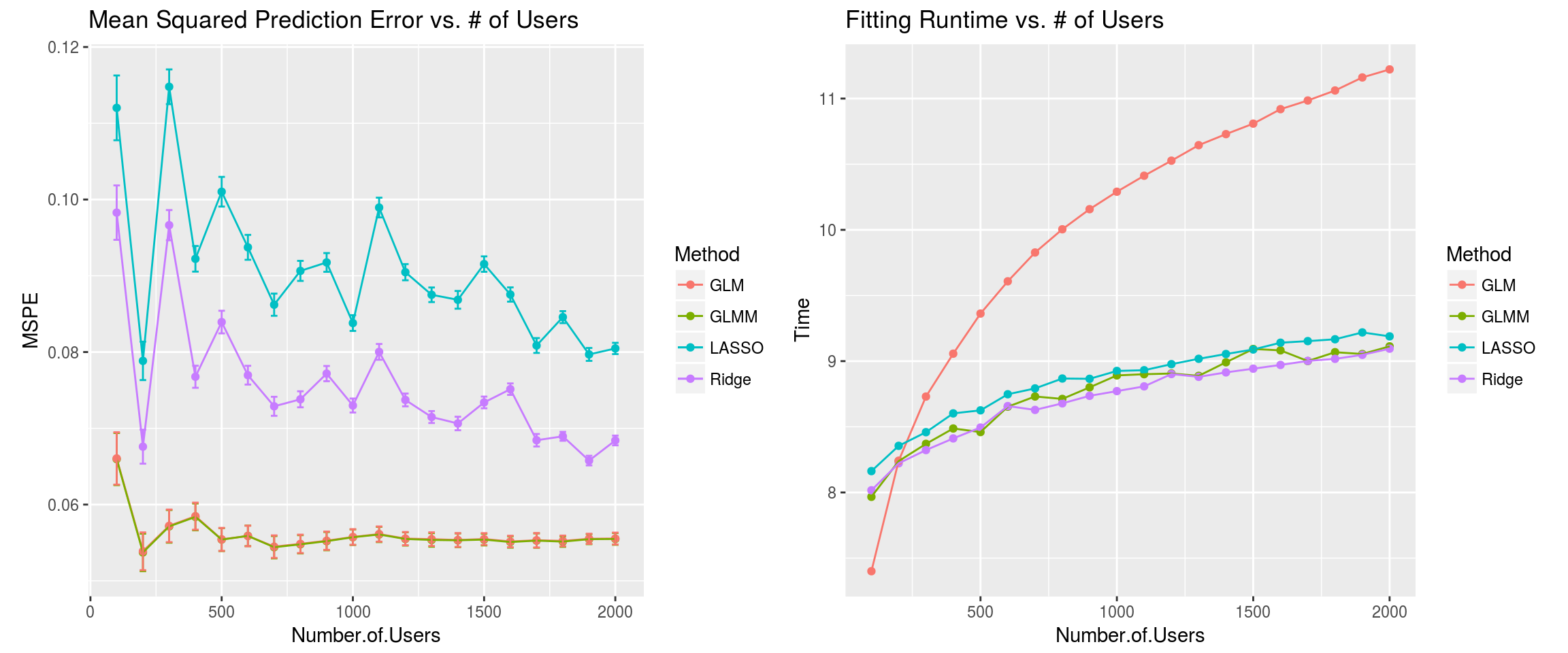
Some conclusions:
The LASSO and Ridge models are worse than the GLM and GLMM models. Possibly, the model parsimony provided by the former methods is actually harmful in this setting. This result possibly reflects the same phenomenon at play in the Google blog post.
The MSPEs of the GLM and GLMM fits are nearly identical. This should not be surprising, since the model matrix equations are essentially the same.
While GLM and GLMM fits are identical, we seem to be gaining something computationally by fitting a mixed-effects model. This is probably only due to the particular R packages involved. Specifically, I think the fact that the GLM estimates come with standard errors is the main bottleneck. If we just cared about prediction, there is probably an equally fast GLM implementation. That being said, the choice to disregard user effects as parameters of interest provided the additional benefit of a faster off-the-shelf solution.
Summary
In the first example, the Lannister family helped demonstrate dealing with multiple experimental units. This is a classical statistical concept that is still extremely relevant in many present-day applications. When we care to estimate the variance of the unit effect population, but not the effects themselves, mixed effects models are a great choice.
Parameter randomness in mixed effects models has a different interpretation than parameter randomness in Bayesian models. In fact, you can take any combination of a (fixed-effect/mixed-effect, Bayesian/frequentist) approach to modeling parametric data.
In a realistic simulation setting with large numbers of experimental units, a mixed-effect approach out-performed some industry-standard fixed-effect approaches with respect to prediction error on future data from the same simulation procedure. Cool!
Caveats:
For the fixed-effect models, there might be better rules-of-thumb or different regularization techniques that would make more sense for situations like the CTR example. Maybe these would improve their performance, but I’m not sure. The results shown are from the most straightforward off-the-shelf implementations for some of the most common regularization approaches.
Wait, you work at Google, why are you responding to one of their blog posts on a personal blog? I wrote this post before I got the job (almost a year before my first day), and published it on my old webpage. I recently completely revamped my website and blogging workflow (everything uses blogdown now), so I’m using this as an easy “first” post. As mentioned at beginning, I just tweaked the writing style; the analysis is unchanged. I think it’s still a good reference for these very general methods, and I’ve gone back to it a few times myself!
Further reading and references:
- http://glmm.wikidot.com/faq
- http://datascienceplus.com/introduction-to-bootstrap-with-applications-to-mixed-effect-models
- http://www.ats.ucla.edu/stat/r/dae/melogit.htm
- Variance Components (Searle, Casella, and McCulloch, 1992)
- Generalized Linear Models, 2nd Edition (McCullagh and Nelder, 1989)
Code examples:
To make the CTR simulation data:
make_click_data <- function (p, # Number of people to choose
                             mu, # Baseline logit-probability of click
                             tau, # Effect of new display
                             sig_a, # Variance of random effects
                             pois_mean, # Mean number of impressions
                             effects = NULL) { # In case you actually want to fix effects

  if (is.null(effects))
    effects <- rnorm(p, 0, sig_a)

  # Preparing design
  treat <- rbinom(p, 1, 0.5)
  treat_expos <- rpois(p, pois_mean * 0.5) + 1
  null_expos <- rpois(p, pois_mean * (1 - 0.5)) + 1
  id <- 1:p
  expos <- treat_expos + null_expos
  expos <- c(expos[!treat == 1], null_expos[treat == 1], treat_expos[treat == 1])
  id <- c(id[!treat == 1], rep(id[treat == 1], 2))
  treat <- c(treat[!treat == 1], rep(0, sum(treat)), rep(1, sum(treat)))
  means <- mu + treat * tau + effects[id]
  probs <- exp(means) / (1 + exp(means))

  # Getting response and making data matrix
  Y <- rbinom(length(probs), expos, probs)
  dataMat <- data.frame("clicks" = Y,
                        "expos" = expos,
                        "display" = treat,
                        "id" = as.factor(id))

  return(list("Data" = dataMat,
              "Effects" = effects))

}

# Make simulated data
set.seed(1)
CTR_Exp1 <- make_click_data(p = 1e3,
                            mu = -4.5,
                            tau = 0.5,
                            sig_a = 5,
                            pois_mean = 20)
To calculate MSPE of the methods over many repetitions of the data from the original simulation model:
user_effects <- CTR_Exp1$Effects
nsims <- 50
MSEP_mat <- matrix(0, 4, nsims)
rownames(MSEP_mat) <- c("GLMM", "LASSO", "Ridge", "GLM")
for (i in 1:nsims) {

  # Generating data
  new_CTR <- make_click_data(p = 1e3,
                             mu = -4.5,
                             tau = 0.5,
                             sig_a = 5,
                             pois_mean = 20,
                             effects = user_effects)

  # Prepping LASSO data
  new_id.matrix <- sparse.model.matrix(~ new_CTR$Data$id - 1)
  new_Sparse.Data <- cBind(new_id.matrix, new_CTR$Data$display)

  # Getting y data
  new_weights <- new_CTR$Data$expos
  new_nclicks <- new_CTR$Data$clicks
  y_new <- unname(cbind(new_weights - new_nclicks, new_nclicks))

  calc_MSEP <- function (pred) {
    err0 <- pred^2 * y_new[ , 1]
    err1 <- (1 - pred)^2 * y_new[ , 2]
    return((sum(err0) + sum(err1)) / sum(new_weights))
  }

  # Calculating prediction logit means
  lme_pred <- predict(CTR_lme1, newdata = new_CTR$Data)
  lasso_pred <- predict(CTR_lasso, newx = new_Sparse.Data)
  ridge_pred <- predict(CTR_ridge, newx = new_Sparse.Data)
  glm_pred <- predict(CTR_glm, newdata = new_CTR$Data)

  # Calculating prediction probs
  lme_pred_probs <- exp(lme_pred) / (1 + exp(lme_pred))
  lasso_pred_probs <- exp(lasso_pred) / (1 + exp(lasso_pred))
  ridge_pred_probs <- exp(ridge_pred) / (1 + exp(ridge_pred))
  glm_pred_probs <- exp(glm_pred) / (1 + exp(glm_pred))

  # Calculating prediction probs
  prob_mat <- cbind(exp(lme_pred) / (1 + exp(lme_pred)),
                    exp(lasso_pred) / (1 + exp(lasso_pred)),
                    exp(ridge_pred) / (1 + exp(ridge_pred)),
                    exp(glm_pred) / (1 + exp(glm_pred)))

  MSEP_mat[ , i] <- unname(apply(prob_mat, 2, calc_MSEP))

}
The MSPE in this setting is defined as follows: Let \(\hat\mu_{ij}\) be the model-predicted logit-mean for that user-display combination. Let \(\hat p_{ij} = \frac{\exp\{\hat\mu_{ij}\}}{1 + \exp\{\hat\mu_{ij}\}}\), which is the model-predicted probability of the \(j\)-th user interacting with display version \(i\). Let \(y_{ijk}^\ast\) be the \(k\)-th new data point from the \(j\)-th user seeing display version \(i\). Let \(n^\ast_{ij}\) be the number of times the \(j\)-th user saw display \(i\), and define \(N^\ast:=\sum_{ij}n^\ast_{ij}\). Then: \[ \text{MSPE} := \frac{1}{N^\ast}\sum_{ij}\sum_k(y^\ast_{ijk} - \hat p_{ij})^2 \]↩